1. General:
|
After installation you should periodically check the latest news about FactSage 7.1
where we immediately report any 'bugs' and other issues as they surface - www.FactSage.com > 'FactSage 7.1 ~ News ~' |
FactSage 7.1 ~ News ~ |
The 'bugs' and other issues highlighted in the previous 'FactSage 7.0 ~ News ~' have been resolved.
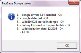
FactSage dongle status
- When a valid HASP dongle is attached to a USB port on the computer you are able to run a standalone version
of FactSage.
If FactSage issues an error message about a 'missing or invalid FactSage HASP security key'
it goes into the FactSage SetUp mode with a green screen.
There are several factors that can cause this to happen.
The 'FactSage dongle status' Window shown here is for an installation where a valid FactSage dongle
is attached and everything is in order (i.e. 1 - 5. All OK).
You can update/refresh a FactSage Standalone computer or a Network
Server. In the case of a network installation it is
only necessary to update/refresh the Network Server.
Do not update a FactSage 6.4 installation -
in this case select 'New Factsage installation' and install FactSage 7.1 in a new folder.
A new publication (Paper III) has been added to the list and can be displayed on the computer screen -
"FactSage thermochemical software and databases, 2010 - 2016", CALPHAD, Vol. 54, pp. 35-53, 2016.
FactSage-TEACH is a selftuition package on FactSage developed by GTT-Technologies.
It is combination of a special handbook, a series of special mini-databases for use with the assignments,
and a special flowsheet model for the Silicon Arc Furnace process.
It is the result of a long series of seminars, training courses and workshops on Computational Thermochemistry
which began in the early nineties using ChemSage.
For more information including the 'Table of Contents' click 'General > FactSage-TEACH > Introduction ...'.
The FactSage-TEACH manual has been revised in FactSage 7.1.
To view the manual click on 'General > FactSage-TEACH > Documentation ...'.
In addition over 50 new phase diagrams (mainly FToxid systems) have been added to the list.
There is a new option in Reaction -
The volume data can be displayed via the View Data module or more simply by a 'mouse-right-click' (or 'mouse-double-click') on the species listed the Reaction Reactants Window.
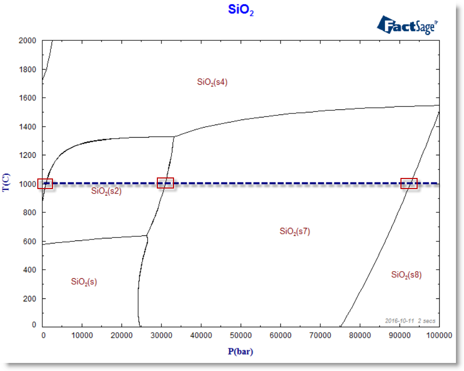
The Phase Diagram and Reaction figures below show the effect of temperature and pressure on the stability of SiO2 phases.
1 - T(C) versus P(bar) phase diagram of SiO2 with 'include volume data' in effect
- the phase transitions at 1000 C are highlighted.
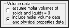
The option 'include molar volume data and physical properties data' takes into account the effect of thermal expansivity
and compressibility data on the molar volume of the species and effects the 'VdP' term used in the calculation.
In addition physical properties such as bulk modulus, Curie temperature, electrical conductivity, thermal conductivity ,
thermal expansivity, viscosity etc. are displayed when available.
The maximum number of selected product solutions is now 150 (was 40 in FactSage 7.0). The maximum number of product species (3000) and product phases (1500) remain unchanged.
This new feature was first introduced in FactSage 7.0 and remains unchanged.
It displays the status of the FactSage dongle attached to the computer.
This helps you to diagnose the source of the error message.
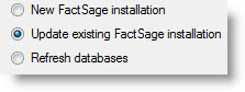
The FactSage 7.1 Installation program enables you to update/refresh FactSage 7.1 software,
documentation and databases to the full FactSage 7.1 package.
You can update a FactSage 7.0 installation.
2. Modules:
- called from 'General > FactSage Documentation ...'.
- called from 'General > FactSage-TEACH ...'.

 - to include volume data for the solids and liquids.
This takes into account the effect of thermal expansivity and compressibility data on the molar volume of the species and effects the 'VdP' term used in the calculation.
The effect of such data is only meaningful in calculations at high pressures.
In Reaction the volume data have no effect on the gas phase - the gas is always treated as ideal.
- to include volume data for the solids and liquids.
This takes into account the effect of thermal expansivity and compressibility data on the molar volume of the species and effects the 'VdP' term used in the calculation.
The effect of such data is only meaningful in calculations at high pressures.
In Reaction the volume data have no effect on the gas phase - the gas is always treated as ideal.
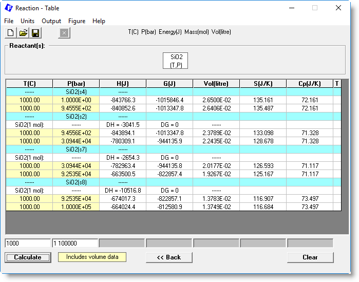
2 - Reaction Table Window showing the effect of P on the phase transitions of SiO2 at 1000 C with 'include volume data' in effect.
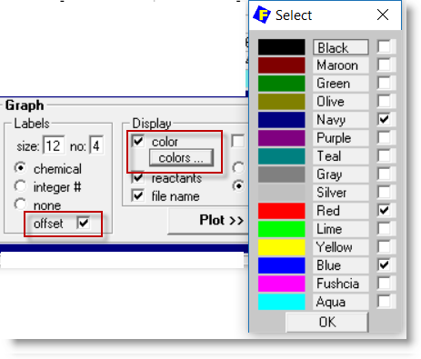
SET PLOT AXIS/CAPTION/LABELS/DISPLAY/SELECT:

SET PLOT AXIS Y-AXIS (X-AXIS) a (n  etc.) Y (log10(Y) ln(Y) ...) 'minimum' 'maximum' 'step'

SET PLOT CAPTION TITLE    'figure title'                 // Figure title
SET PLOT CAPTION SUBTITLE 'figure sub-title'             // and subtitle
SET PLOT CAPTION Y-TITLE (X-TITLE) 'axis title'          // Axes captions
SET PLOT CAPTION LABEL     'X coordinate' 'y coordinate' "label #1"  // User-defined labels
SET PLOT CAPTION LABEL     'X coordinate' 'y coordinate' "label #2"  //
SET PLOT CAPTION LABEL      .... etc.                                //

SET PLOT LABELS  SIZE  2 (2 - 24)           // size of labels  (Post Processor Window)
SET PLOT LABELS  NO    2 (1 - 9)            // number per line
SET PLOT LABELS  CHEMICAL [INTEGER or NONE) // type of label
SET PLOT LABELS  OFFSET       ON (OFF)      // offset labels above the coordinate

SET PLOT DISPLAY COLOR        ON (OFF)      // line color on (or B/W)      (Post Processor Window)
SET PLOT DISPLAY COLORS  9 12 2             // line colors 0 - 14          (Post Processor Window)
SET PLOT DISPLAY COLORS  RED BLUE GREEN     // line color names BLACK MAROON ... AQUA
//          0 = BLACK, 1 = MAROON, 2 = GREEN, 3 = OLIVE, 4 = NAVY,   5 = PURPLE, 6 = TEAL,
//          7 = GRAY,  8 = SILVER, 9 = RED,  10 = LIME, 11 = YELLOW, 12 = BLUE, 13 = FUSHIA, 14 = AQUA

SET PLOT DISPLAY REACTANTS    ON (OFF)      // list reactants in the title   (if CAPTION TITLE not set)
SET PLOT DISPLAY FILE_NAME    ON (OFF)      // list source file in subtitle (if CAPTION SUBTITLE not set)

SET PLOT DISPLAY SOURCE       ON (OFF)      // include data source in species label (Plot Species Selection Window)
SET PLOT DISPLAY PHASE        ON (OFF)      // include phase name in species label
SET PLOT DISPLAY NAME         ON (OFF)      // include species name in species label
SET PLOT DISPLAY PAGE         ON (OFF)      // include page number in species label

SET PLOT SELECT  CLEAR                      // clear current species selection
SET PLOT SELECT  MASS    MOLE (GRAM)        // mass units
SET PLOT SELECT  ORDER   INTEGER (MASS FRACTION or ACTIVITY) // order with respect to integer or mass ...
SET PLOT SELECT  TOP     1 (2 ....)                          // select top species as defined in ORDER
SET PLOT SELECT  IGNORE  ON (OFF)                            // ignore species and phase that have no mass
SET PLOT SELECT  STABLE  PHASE (LIQUID SOLID SOLUTION)       // select all stable phases (all s table pure liquids ...)
SET PLOT SELECT  SPECIES 2 5 8                               // select species 2 5 and 8
3. Set Activity - EquiEx_CH4-O2_Set-Activity.mac
There is a new macro file, EquiEx_CH4-O2_Set-Activity.mac, that shows how to define the equilibrium P(O2(g)) and a(C(s)) in a system.
The macro :
opens the stored example Ex_CH4-O2.dat - CH4 (25C,gas) + (alpha) O2 (25C,gas) => Adiabatic identifies O2(g) as an 'ACTIVITY species' and sets P(O2) equilibrium = 1e-5 redefines the amounts of reactant CH4 and O2, defines the final temperature 1600, and defines Delta H (Z) = 'blank' (i.e. the reaction is no longer adiabatic) calculates the equilibrium and displays the results where P(O2) = 1e-5 drops P(O2) from the ACTIVITY calculation identifies C(s) as a new 'ACTIVITY species' and defines equilibrium range of values of log(a(C)) = -5 -4 -3 and -2 calculates the equilibrium and displays the results where a(C) = 1e-5, 1e-4, 1e-3 and 1e-2
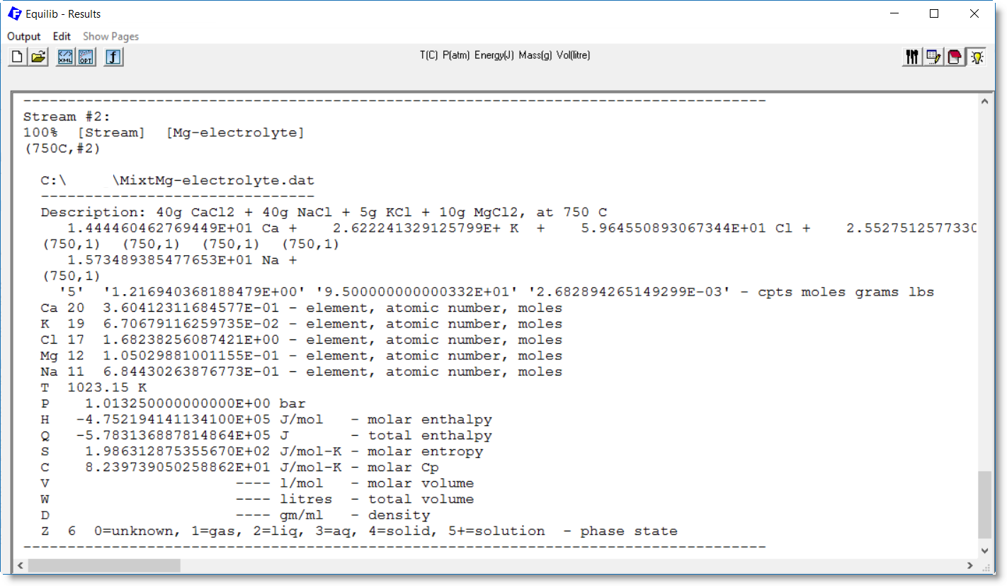
4. [Streams]
In Macro Processing a [stream] (MIXT*.dat file) is often created and then used (recycled) as input for the next part of the simulation. Sometimes the same EQUI*.dat file containing particular [streams] is repeatedly opened in order update the new [stream] values.
In FactSage 7.1 when a [stream] is updated it is no longer necessary to re-OPEN the same Equilib file. Before the equilibrium is calculated (CALC command) the program first checks to see if the MIXT*.dat file has been updated. If necessary the program automatically refreshes the input values and only then calculates the equilibrium.
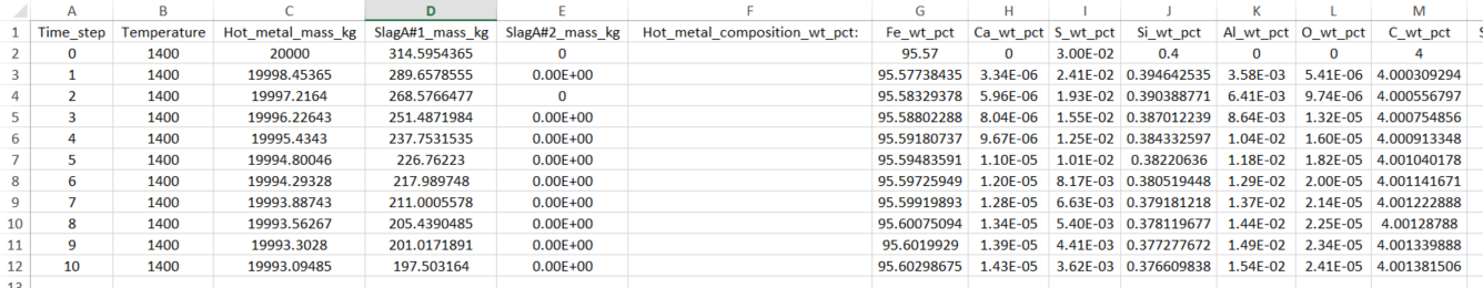
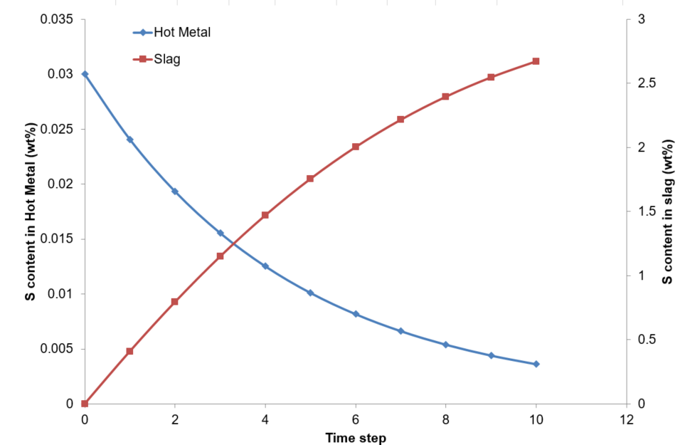
Macros and Recycling [Streams]An example of recycling [streams] is given in the new macro file EquiEx_Streams.mac that is stored in the folder Macros\Ex_Streams. The example shows how to use streams in a simplified steelmaking process. The process consists of the desulfurisation of hot metal by the top slag.
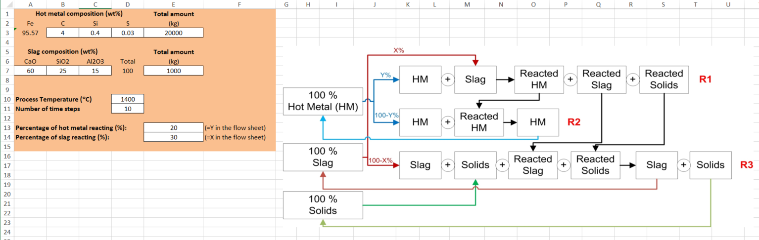
The process is broken down into 3 reactions:
A fraction of the hot metal is equilibrated with a fraction of the slag in R1
In R2, the hot metal product from R1 is mixed back with the remaining hot metal
In R3, the slag products from R1 (including liquid slag and pure compounds) are mixed with the remaining top slag Each phase (i.e. hot metal, liquid slag and pure compounds) is saved in a [stream] and passed to the next Equilib file or to the next time step Reactions R1, R2 and R3 are repeated at each time step, until the total process duration is reached.
In FactSage 7.1 all known bugs have been fixed and the program stability has been improved.
All the FactOptimal examples have been thoroughly checked and revised where necessary.
FactOptimal can now be coupled with the Viscosity module in order to calculate
the compositions and temperatures that maximise, maximise or target a viscosity under a certain set of constraints on composition.
See Viscosity below for details.
Details are given below in the section 3. Phase Diagram Variables Window.
Classical Eh-pH (Pourbaix) diagrams are not true phase diagrams and have been replaced by Aqueous Phase Diagrams
(see below for more details).
That is, it is no longer possible to calculate the classical Eh versus pH (Pourbaix) diagram in the Phase Diagram module.
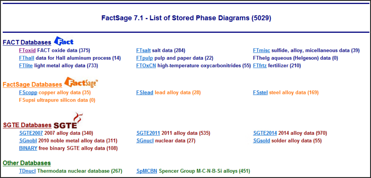
Approximately 70 example diagrams with various X- and Y-axes are stored in Phase Diagram.
Examples of Aqueous Phase Diagrams and Scheil-Gulliver Constituent Diagrams (see below) have been added to the list.
To display a summary (htm format) of all these diagrams
click on 'Phase Diagram > Components Window > Help > Phase Diagrams with various ...'.
To load and calculate the various phase diagrams
click on 'Phase Diagram > Components Window > File > Directories > Phase diagrams with various ...'.
This list of examples is by no means exhaustive.
2. Phase Diagram Menu Window
The maximum number of selected product solutions is now 150 (was 40 in FactSage 7.0). The maximum number of product species (3000) and product phases (1500) remain unchanged.
3. Phase Diagram Variables Window - 'Phase Diagram > Menu Window > Variables ...'
In FactSage 7.0 for the ternary system A-B-C you can plot T vs A/(A+B+C) at a constant composition C/(A+B+C).
In the quaternary system A-B-C-D you can calculate the Gibbs phase diagram of A-B-C where the composition variables are A (B and C)/(A+B+C) and the constant composition = D/(A+B+C).
In both systems the composition denominator, (A+B+C). is fixed.
In FactSage 7.1 you can now have a variable composition denominator for the constant.
For example, in the ternary system A-B-C you can plot T vs A/(A+B) at a constant composition C/(A+B+C),
or T vs A/(A+B+C) at a constant composition C/(A+B), and so one.
In the quaternary system A-B-C-D you can now calculate the Gibbs phase diagram of A-B-C where the composition variables are A (B and C)/(A+B+C) and the constant composition is D/(A+B+C+D).
Although the denominator for a constant composition variable may be any expression, when both x- and y-axes are
composition variables, then these denominators must be the same.
In FactSage 7.0 for the Fe-Mn-C ternary system where X(Mn) = Mn/(Fe+Mn+C) and X(C) = C/(Fe+Mn+C) you can plot X(Mn) versus X(C) at a constant temperature.
In FactSage 7.1 you can now specify log10(composition) variables.
For example, in the Fe-Mn-C ternary system you could also plot log10(X(Mn)) versus X(C) or log10(X(Mn)) versus log10(X(C)) or log10(X(Mn)) versus log10(X(C)).
Classical Eh-pH (Pourbaix) diagrams are not true phase diagrams inasmuch as
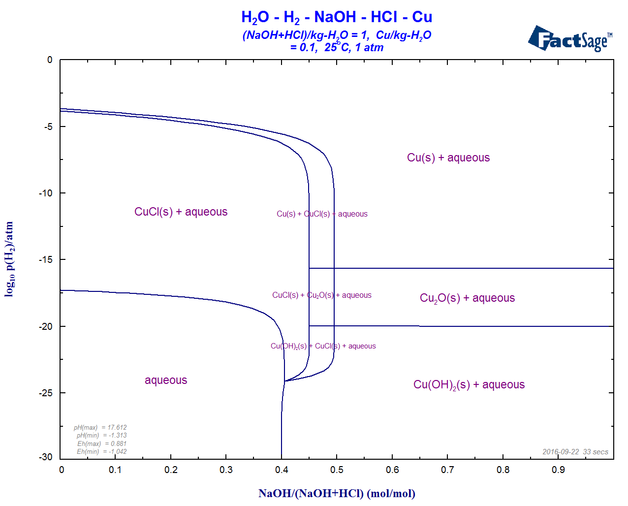
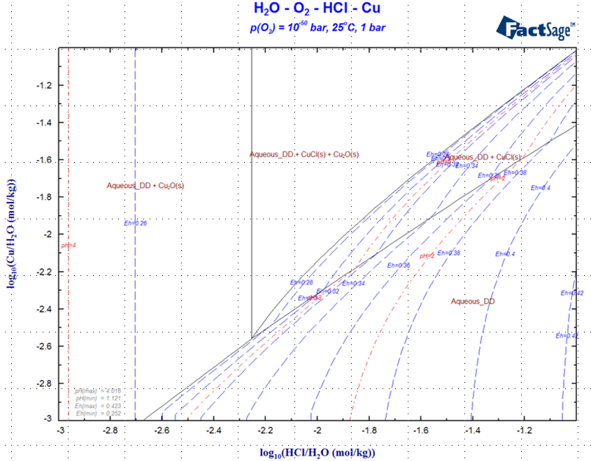
The Aqueous Phase Diagram is a new type of phase diagram in FactSage 7.1 that we have developed for
displaying phases in equilibrium with the aqueous phase.
The figure below shows a calculated phase diagram for the system H2O-Cu-NaOH-HCl-H2
in which the X-axis is the molar ratio NaOH/(NaOH+HCl) (which is related to the pH)
and the Y-axis is the equilibrium partial pressure of H2 (which is related to the redox potential Eh).
The figure is calculated on the basis of 1.0 kg H2O and a total of 1.0 mol (NaOH+HCl) at
a copper content of Cu/(kg-H2O) = 0.1.
The figure shows the stable phases in equilibrium with the aqueous phase.
The composition of the aqueous phase at any coordinate can be calculated by simply placing the cursor at a point on the diagram and clicking.
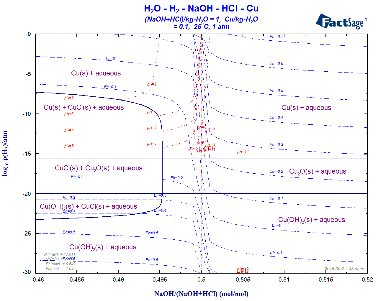
Aqueous Phase Diagrams of the H2O-Cu-NaOH-HCl-H2 - log10(P(H2) versus molar ratio NaOH/(NaOH+HCl) at m(Cu) = 0.1.
In the diagram the X-axis is expanded around 0.5.
The figure includes the calculated iso-Eh and iso-pH lines and illustrates shows the
classical 'titration curve' behavior around equimolar NaOH/HCl.
Aqueous Phase Diagrams with the FThelg non-ideal aqueous solution
During cooling of an alloy from the liquid state at complete thermodynamic equilibrium, all solid solution phases remain homogeneous through internal diffusion and all peritectic reactions proceed to completion.
The stable phases at various compositions and temperatures can be represented by a classical temperature versus composition phase diagram for example as calculated by the Phase Diagram module.
In practice, conditions for cooling often approach more closely to those of Scheil-Gulliver cooling in which solids, once precipitated, cease to react with the liquid or with each other, there is no diffusion in the solids, the liquid phase remains homogeneous, and the liquid and surfaces of the solid phases are in equilibrium.
The Scheil-Gulliver Constituent Diagram is a new type of phase diagram in FactSage 7.1 that we have developed for
displaying the cooling path when a system is cooled and the constituents in the phases are not allowed to diffuse.
Details on Scheil-Gulliver Constituent Diagrams are given in the updated Phase Diagram Slide Show (new slides 18.1 - 18.20)
as well as in a recent publication Scheil-Gulliver Constituent Diagrams by A.D. Pelton, G. Eriksson and C.W. Bale submitted to Met. Trans B, September 2016
(click on 'Slide Show > Phase Diagram - Article - Scheil-Gulliver Constituent Diagrams pdf' )
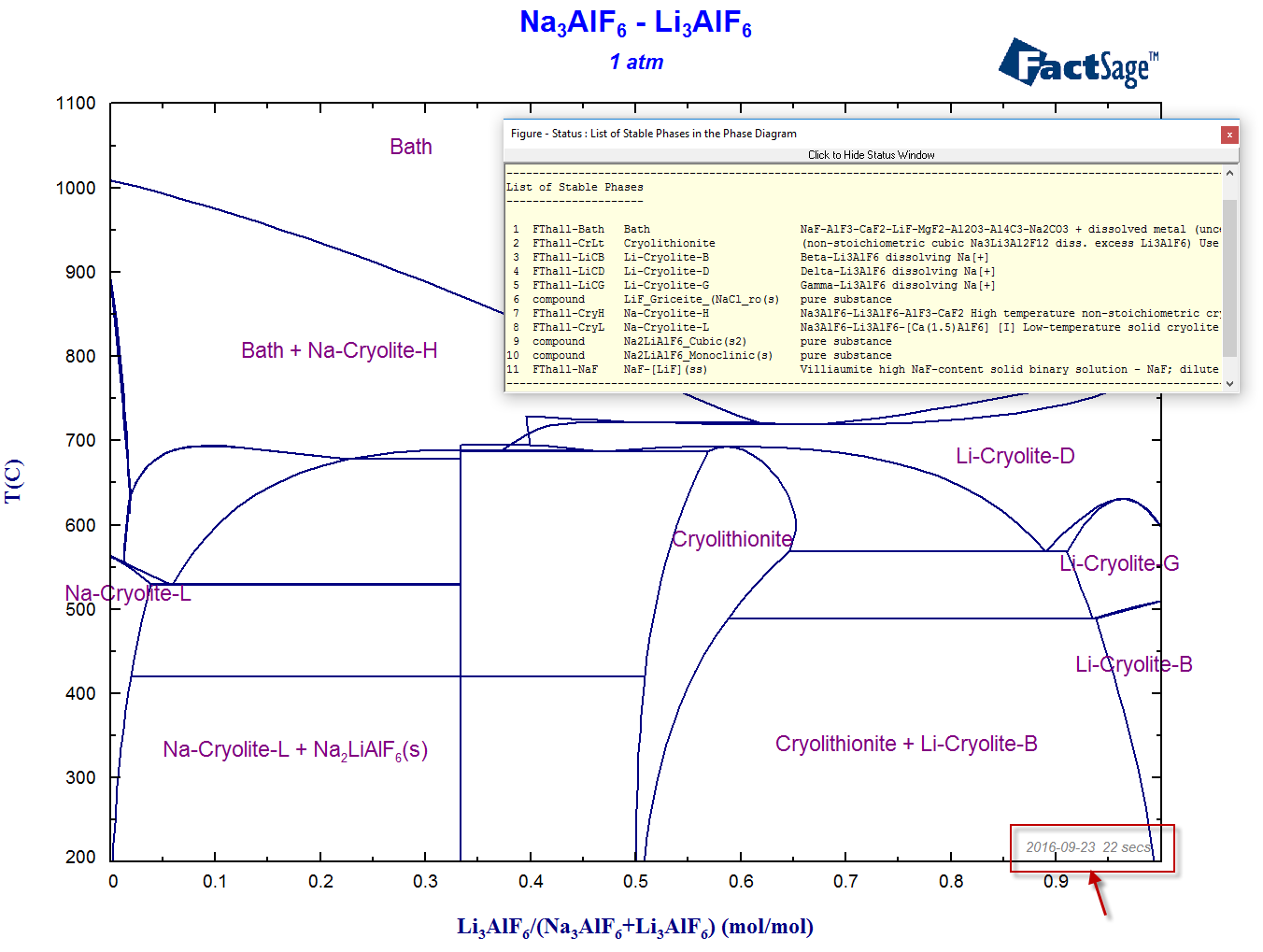
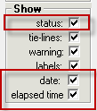
In the Parameters Window the Show options have been enhanced.
After the phase diagram has been calculated:
- the status box now displays Information on the Stable Phases
- the new date and elapsed time options post these values in the lower right corner of the figure
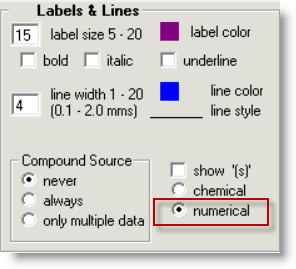
In the Parameters Window the Labels & Lines options
enable you to label the phases by numbers.
This is useful in systems containing many phases.
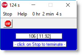
In FactSage 7.1 there are some new features in the Stop Window:
- The Stop Window includes the total elapsed time in seconds as well as hr-min-sec.
- The current calculation step (106) and step elapsed time (11.92 sec) are posted in the window - these are taken from the Figure Status Window.
- the Stop icon
- When the 'Stop' is pressed in the Stop Window, the program terminates the phase diagram calculation as soon as possible.
- When done it posts the message 'Stop button pressed' in the Status Window and also adds the text
'~ Stop button pressed ~' at the bottom of the figure.
- The figure stays active - that is you can still add labels, edit text and perform detailed point calculations in the usual manner.
- When done you can save the Phas*.dat file and its (incomplete) calculated phase diagram in the Menu Window in the usual manner.
In FactSage 7.1 it is now possible to call FactOptimal from within the Viscosity module and calculate
the composition of a system that minimizes, maximizes or targets the viscosity within a set of
constraints on temperature and composition.
The new Slide Show - 'Viscosity and FactOptimal' - includes a worked example that locates the composition
and temperature which minimizes the viscosity of
the system SiO2 - Al2O3 - CaO - MgO,
in the temperature range is 1400 oC - 1800 oC
where the composition constraints are 0.25 < X(SiO2) < 0.5 and X(CaO)+X(MgO) < 0.5
Note that FactOptimal has limited functionalities when called by Viscosity.
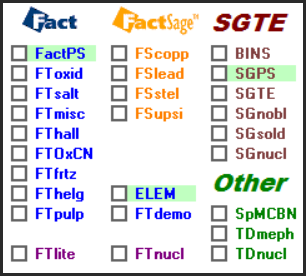
All the public solution databases have been converted to the
new solution database format.
In the FactSage Main Menu click on 'Documentation' for detailed information on the public compound and solution databases.
Due to conflicts within some of the programs, deuterium, D, and tritium, T, have dropped from
FactPS.
(This was done in FactSage 7,0 but it was not reported at the time.)
Data for the following compounds have been updated:
No updates relative to FactSage 7.0.
No updates relative to FactSage 7.0
No updates relative to FactSage 7.0
The CaO-MgO-NiO-SiO2 system has been reoptimized. The changes are
mostly in the Slag, Monoxide, Melilite, Clino-Pyroxene, Proto-Pyroxene
and Olivine solutions
The whole BaO-Al2O3-B2O3-CaO-MgO-SiO2 system has been optimized, including 15
solid solutions and numerous stoichiometric compounds.
The Na2O-FeO-Fe2O3-Al2O3-SiO2 system has been optimized.
The following solutions have been updated: Slag, Monoxide, Clino-pyroxene,
Mullite, Carnegieite, Nepheline, low- and high-T Meta-aluminate/ferrite
(NASl and NASh), Feldspar and beta"-alumina.
ZrO2-containing binaries and ternaries from the
Al2O3-CaO-MgO-SiO2-ZrO2 system have been reoptimized, as well as the
MnO-ZrO2 binary. Slag, Monoxide and ZrO2-based solid solutions (cubic,
tetragonal, monoclinic) have been updated.
The FToxid compound database now includes the volumetric and thermal conductivity
parameters for 52 compounds.
There are also a few minor updates/corrections in several solid
solutions and compounds.
Over 50 new FToxid phase diagrams have added to the 'list of stored phase diagrams'.
- Revision of the Fe-Ti-C system.
Better description of TiC formation.
- Revision of the Al-Fe-Zn system.
Inconsistency of Al-Fe-Zn system for Zn galvanizing calculation is resolved.
What's New in:

FactOptimal was first introduced in FactSage 6.1.
The module computes optimal conditions for material and process design by coupling FactSage with the Mesh Adaptive Direct Search (MADS)
algorithm for nonlinear optimization developed by the GERAD research group at the Ecole Polytechnique de Montréal.
1. Phase Diagram Components Window
It is now possible to calculate Scheil-Gulliver Constituent Diagrams
and Aqueous Phase Diagrams.

(a) the aqueous phase fields show the regions where one aqueous species is predominant,
whereas this is actually only one continuous aqueous phase field,
(b) they are calculated only at infinite dilution.
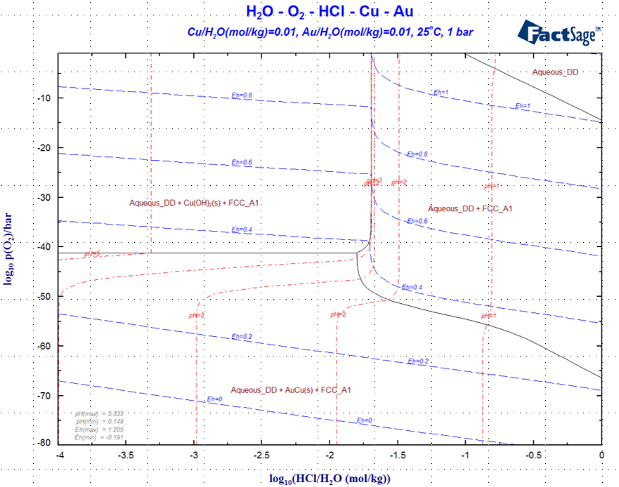
1 - H2O-O2-HCl-Cu-Au aqueous phase diagram involving a non-ideal alloy of Cu and Au where the y-axis is the oxidation potential, log P(O2), which is related to Eh..
2 - H2O-O2-HCl-Cu aqueous diagram with m(HCl) versus log m(Cu) at constant oxygen potential .
Details on Aqueous Phase Diagrams are given in the updated Phase Diagram Slide Show (new slides 19.1 - 19.37).
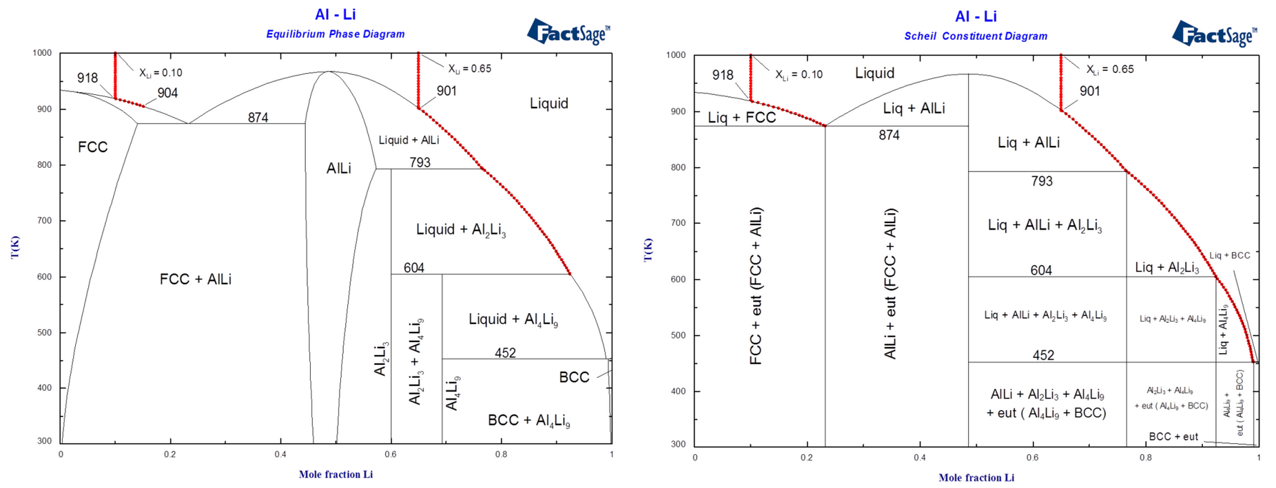
Diagrams of the Al-Li system illustrating solidification of alloys of compositions XLi = 0.10 and XLi = 0.65.
1 - Calculated phase diagram and equilibrium solidification.
2 - Calculated Scheil-Gulliver constituent diagram and Scheil-Gulliver solidification.
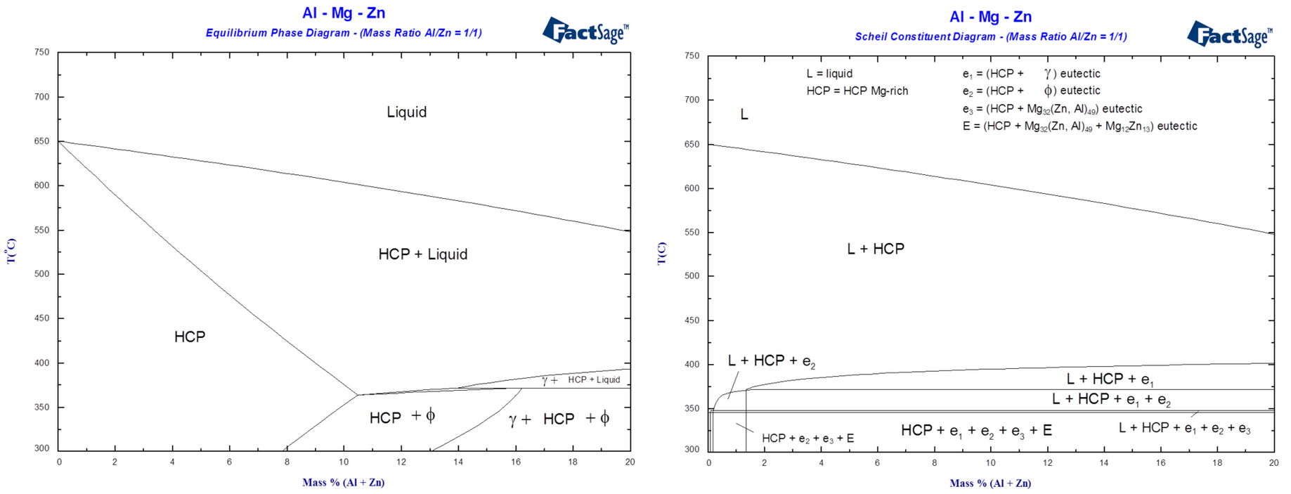
Diagrams of the Al-Mg-Zn ternary system for Mg-rich alloys at constant mass ratio Al/Zn = 1/1
1 - Calculated phase diagram and equilibrium solidification.
2 - Calculated Scheil-Gulliver constituent diagram and Scheil-Gulliver solidification.
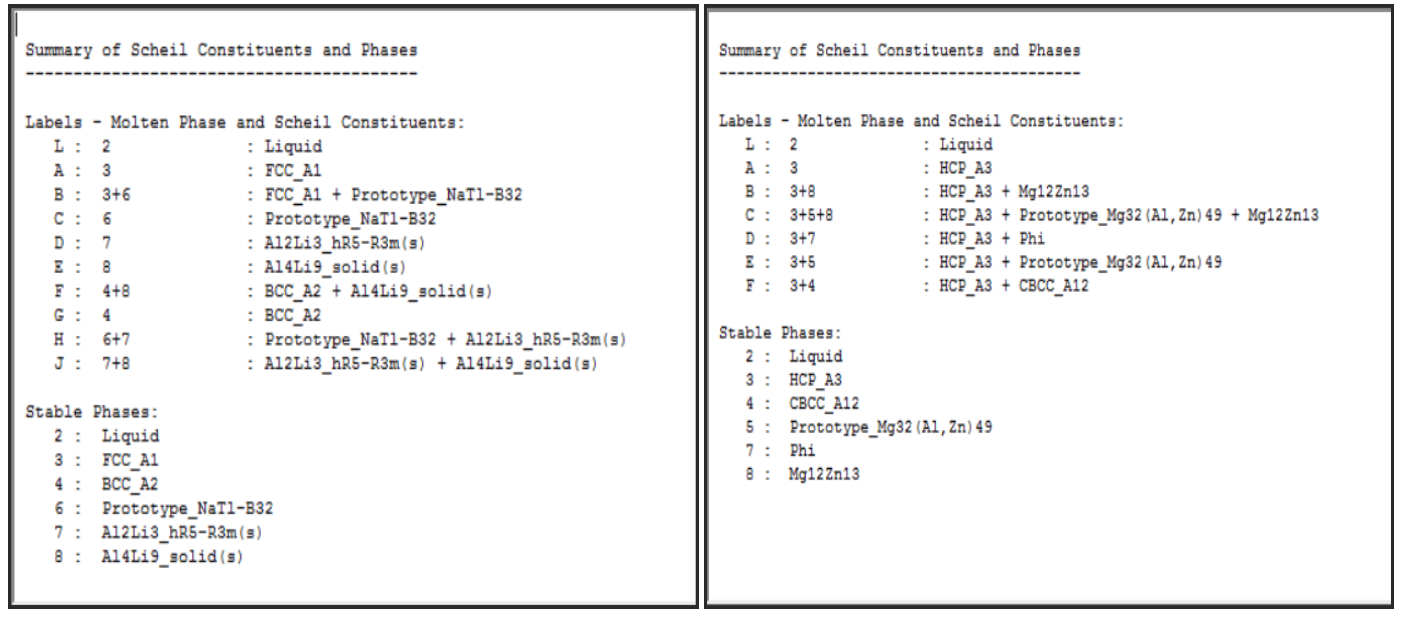
Tables listing the Scheil constituents and phases during Scheil cooling.
1 - Scheil cooling in the Al-Li binary system.
2 - Scheil cooling in the Al-Mg-Zn ternary system..
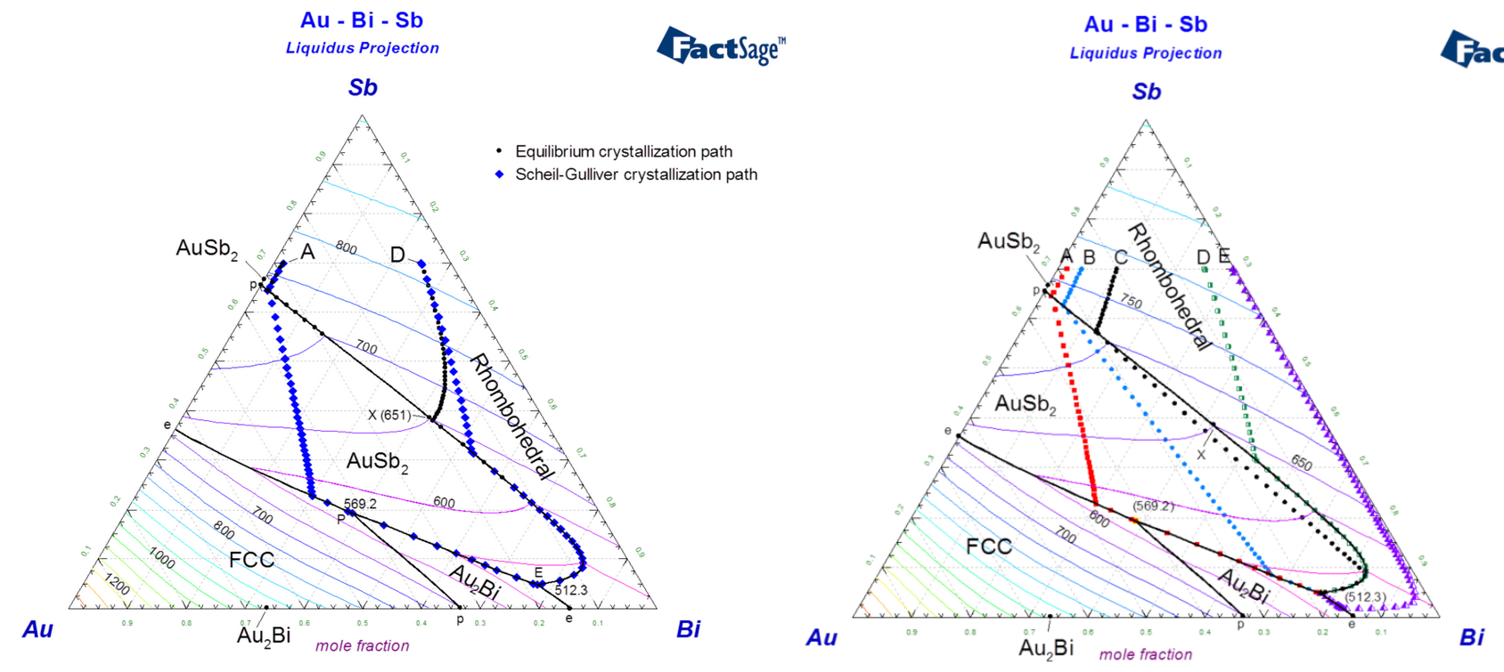
Calculated liquidus projection of the Au-Bi-Sb ternary system.
1 - Crystallization paths during equilibrium cooling (circles) and Scheil-Gulliver cooling (diamonds) are shown for two alloys (A and D).
2 - Crystallization paths during Scheil-Gulliver cooling are shown for five alloys (A, B, C, D, E)
as well as the date and elapsed time (22 secs) of the calculation .
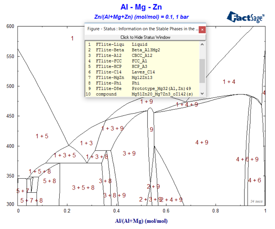
The correspondence between phase number and phase name is given in the 'Information on the Stable Phases'.
You activate the 'Stop Window' via the Parameters Window.
This enables you to terminate a phase diagram calculation at any time without terminating or quitting the Phase Diagram (or Equilib) module..
![]()
The Viscosity module calculates the viscosity of a glass or slag solution at a given temperature and composition.
The FactOptimal module is programmed to identify the optimal conditions for alloy and process design
using thermodynamic and property databases.
C8H10 Ce Dy Er Eu Gd Ho La Lu Nd OPCl3 Pm Pr SbO Sc Sm Tb Tm Y Yb
No updates relative to FactSage 7.0
No updates relative to FactSage 7.0
No updates relative to FactSage 7.0
No updates relative to FactSage 7.0
No updates relative to FactSage 7.0
- Revision of the description of the Fe-Si-C system.
The description of The Fe-Mn-Si-Al-C system for AHSS calculation is improved.
No updates relative to FactSage 7.0
No updates relative to FactSage 7.0
No updates relative to FactSage 7.0
4. Previous FactSage Updates
What's New in: