Click on Download Equilib Regular Slide Show (pdf presentation - 102 pages) for detailed information on the regular features of the Equilib Module. Click on Download Equilib Advanced Slide Show (pdf presentation - 115 pages) for detailed information on the advanced features of the Equilib Module.

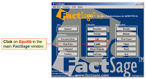
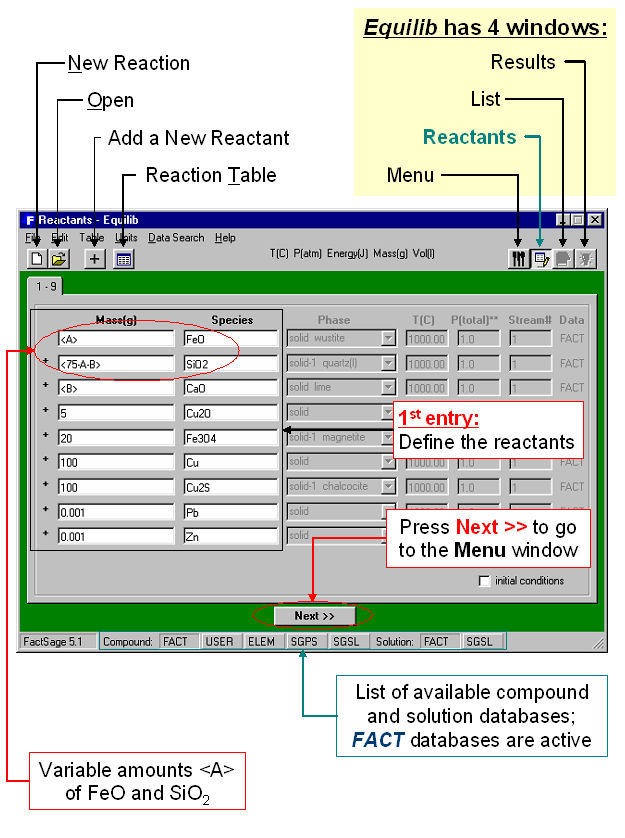
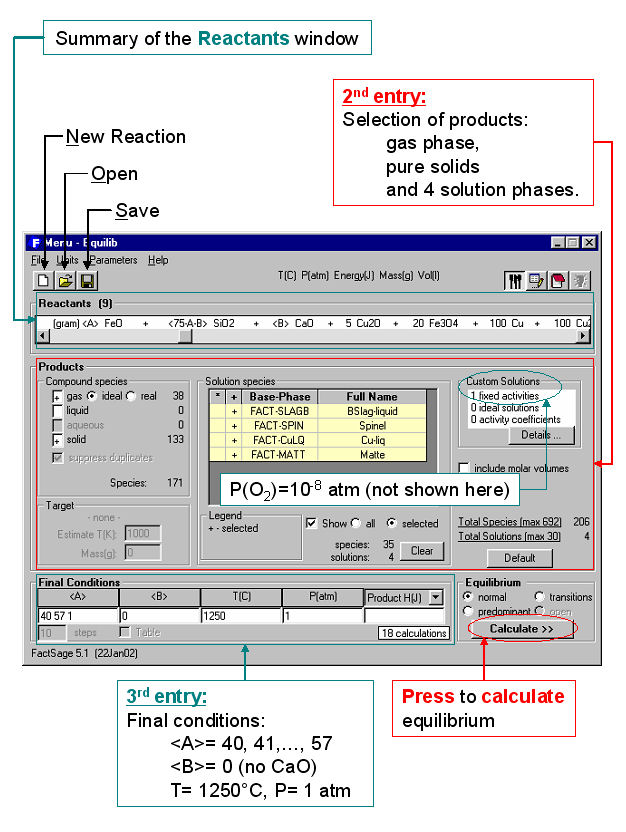
The Equilib module is the Gibbs energy minimization workhorse of FactSage and the most popular program. It calculates the concentrations of chemical species when specified elements or compounds react or partially react to reach a state of chemical equilibrium. In most cases the user makes three entries as shown in the Equilib Reactants Window (Fig. 2) and Menu Window (Fig. 3):

1st entry: Define the reactants, then click on ‘Next >>’. 2nd entry: Select the possible compound and solution products. 3rd entry: Set the final conditions - T and P, or other constraints, then click on ‘Calculate >>’.

The Reactants Window (Fig. 2) shows the entry for a copper-based pyrometallugical system (variable amounts <A> of FeO, <75A – B> of SiO₂, and <B> of CaO, with fixed amounts of Cu₂O, Fe₂O₃, Pb, Zn, Cu and Cu₂S).

In the Menu Window (Fig. 3) the possible products are identified (gas phase, pure solids and slag, spinel, matte, copper alloy solution phases) together with a range of composition (<A> = 40, 41, 42, ... 57), the temperature (1250ºC) and total pressure (1 atm.). Not shown here is how one can set various constraints, options, targets, etc. (in the example the equilibrium partial pressure of oxygen was fixed at P(O₂) = 10^-8 atm). You then click on the “Calculate >>” button and the computation commences.

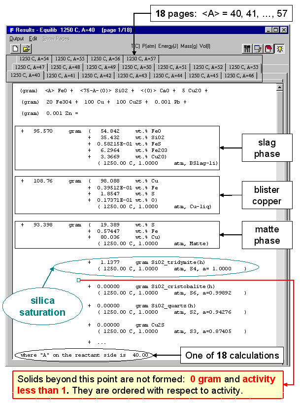
When the calculation is finished you are automatically presented with the Results Window where Equilib provides the equilibrium products of the reaction and where the results may be displayed in F*A*C*T and ChemSage output formats. The equilibrium product amounts are positive, satisfy the mass balance constraints with respect to the system components and correspond to the lowest possible Gibbs energy for this particular selection of possible products. For example Fig. 4 displays the results in F*A*C*T format at <A> = 40; this equilibrium point corresponds to silica saturation, a(SiO₂) = 1.0. The equilibrium compositions of the slag, matte and blister copper are also listed. 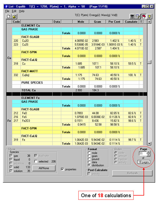Fig. 5 shows a ChemSage output format for <A> = 57 that now corresponds to spinel saturation. The calculated values may also be presented and manipulated via the List Window. For example Fig. 6 shows the distribution of the elements (Cu, Fe) among the phases when <A> = 50.

You may enter up to 48 reactants consisting of up to 32 different components (elements and electron phases). Reactants may include “streams” - these are equilibrated phases stored from the results of previous calculations (useful in process simulation). Phases from the compound and solution databases are retrieved and offered as possible products in the Menu Window. These may include pure substances (liquid, solid), ideal solutions (gas, liquid, solid, aqueous) and non-ideal solutions (real gases, slags, molten salts, mattes, ceramics, alloys, dilute solutions, aqueous solutions, etc.) from the databases described earlier.

Equilib employs the Gibbs energy minimization algorithm and thermochemical functions of ChemSage and offers great flexibility in the way the calculations may be performed. For example, the following are permitted: a choice of units (K, C, F, bar, atm, psi, J, cal, BTU, kwh, mol, wt.%, ...); dormant phases in equilibria; equilibria constrained with respect to T, P, V, H, S, G, U or A or changes thereof; user-specified product activities (the reactant amounts are then computed); user-specified compound and solution data; and much more. Phase targeting and one-dimensional phase mappings with automatic search for phase transitions are possible. For example, you can calculate all equilibrium (or Scheil-Gulliver non-equilibrium) phase transitions as a multicomponent mixture is cooled.

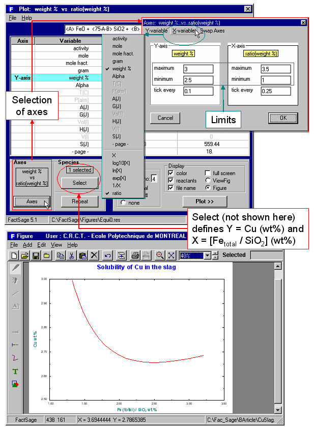
Equilib offers a post-processor whereby the results may be manipulated in a variety of ways: tabular output ordered with respect to amount, activity, fraction or elemental distribution; post-calculated activities; user-specified spreadsheets of f(y) where y = T, P, V, H, S, G, U , A, Cp or species mole, gram, activity, mass fraction and f = y, log(y), ln(y), exp(y) etc. for Lotus 1-2-3, Microsoft Word or Excel. For example Fig. 7 shows post-processing of the results and the generation of a Cu wt%. 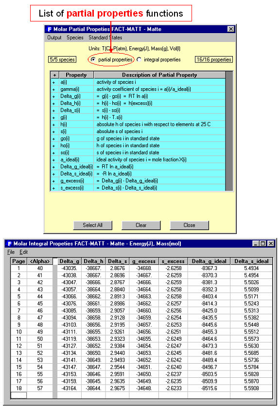vs Fe(total)/SiO₂ wt.% diagram for the complete set (18) of equilibrium calculations. Fig. 8 shows (top) a display of the thermodynamic partial properties functions, and (bottom) a partial listing of the calculated integral properties of a solution phase (FACT-MATT) for all 18 calculations.

Fig. 1 - Equilib Module Fig. 2 - Equilib Module - Reactant Window Cu-matte-slag system. Entry of the rectants including a variable <A> amount of FeO and SiO2. Fig. 3 - Equilib Module - Menu Window Cu-matte-slag system. Selection of possible product phases and definition of the final conditions Fig. 4 - Equilib - Results Window Cu-matte-slag system. Display of the results in F*A*C*T Format for silica saturation (<A>=40). Fig. 5 - EpH - Results Window Cu-matte-slag system. Display of the results in ChemSage Format for spinel saturation (<A>=57). Fig. 6 - Equilib - List Window Cu-matte-slag system. Distribution of the elements (Cu, Fe) among the phases when <A>=50. Fig. 7 - Equilib - Post-processor Window Cu-matte-slag system. Defining and plotting a Cu wt.% vs Fe(total)/SiO2 wt.% diagram for all results (<A>=40 to 57). Fig. 8 - Equilib - Solution Properties Window Cu-matte-slag system. Top: list of the partial properties functions. Bottom: calculated integral properties of the matte phase.