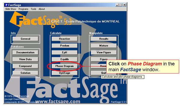
Click on Download
Phase Diagram Slide Show (pdf presentation - 53 pages)
for detailed information on the Phase
Diagram Module.
Phase
Diagram
is a generalized module that permits one to calculate,
plot and edit unary, binary, ternary and multicomponent
phase diagram sections where the axes can be various combinations
of T, P, V, composition, activity, chemical potential,
etc. The resulting phase diagram is automatically plotted
by the Figure module. It is possible to calculate and
plot: classical unary temperature versus pressure, binary
temperature versus composition, and ternary isothermal
isobaric Gibbs triangle phase diagrams; two-dimensional
sections of a multi-component system where the axes are
various combinations of T, P, composition, activity, chemical
potential, etc.; predominance area diagrams (for example
Pso2 vs Po2) of a multicomponent system (e.g. Cu-Fe-Ni-S-O)
where the phases are real solutions such as mattes, slags
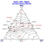
and alloys; reciprocal salt phase diagrams; etc.
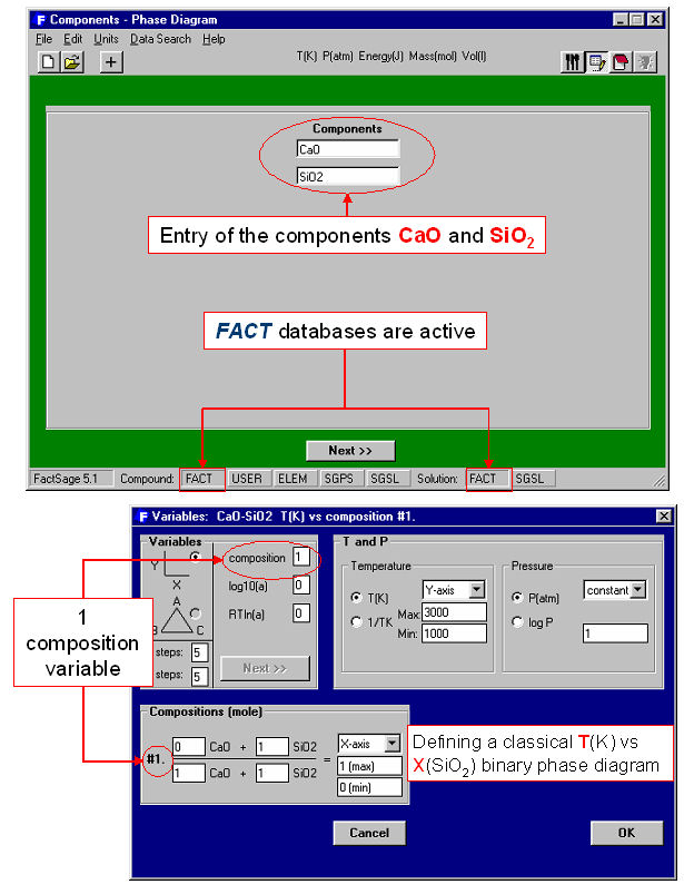
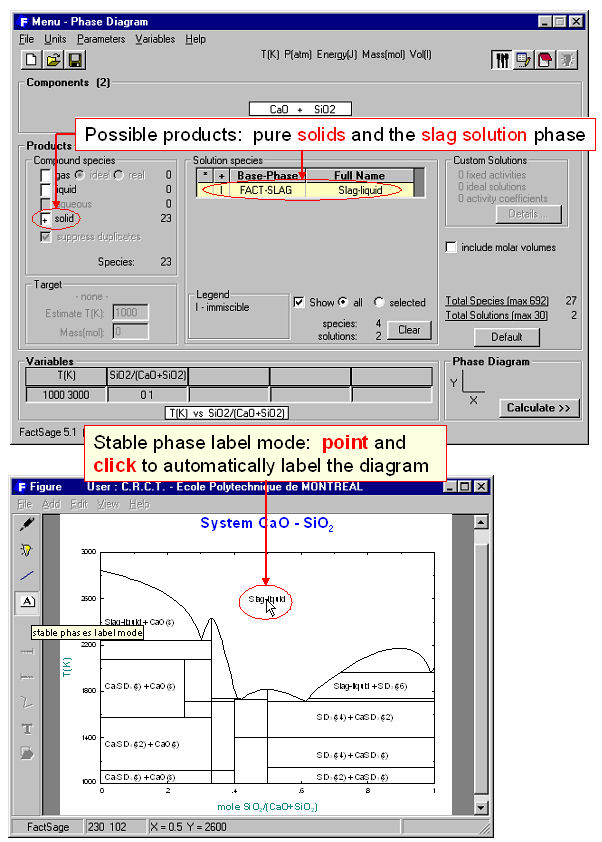
The
calculation of the binary temperature versus composition
phase diagram for the CaO-SiO2 system is shown
in Figs. 2 and 3 In the Phase
Diagram module the system components (CaO,
SiO2) are first entered in the Reactants
Window (Fig. 2 top). Then the type of phase diagram
is defined in the Variables Window (Fig. 2 bottom)
where the user selects the type of diagram (Y vs X, or
Gibbs triangle), the type of axes (composition, activity
and chemical potential), the possible composition variables,
and the limits and constants of the phase diagram. Data
from the compound and solution databases are offered as
possible product phases in the Menu Window (Fig.
3 top). In the case of CaO-SiO2, the slag solution
phase (FACT-SLAG) and all pure solids (including those
outside the plane CaO-SiO2) are selected as
possible product phases. By clicking on the ‘Calculate
>>’ button the phase diagram is automatically
calculated and plotted in real time (Fig. 3 bottom). When
the calculation is complete the Figure
module uses the graph as a dynamic interface. By pointing
to any domain, tie lines and stable phases are automatically
labeled. Optionally the figure can be manipulated: tie
lines can be inserted in the plot, the equilibrium compositions
and phase amounts at any point on the diagram can be calculated
and shown in a table, and the diagram can be edited (add
experimental data points, text, change font and colors
etc.). Examples of edited diagrams are shown later.
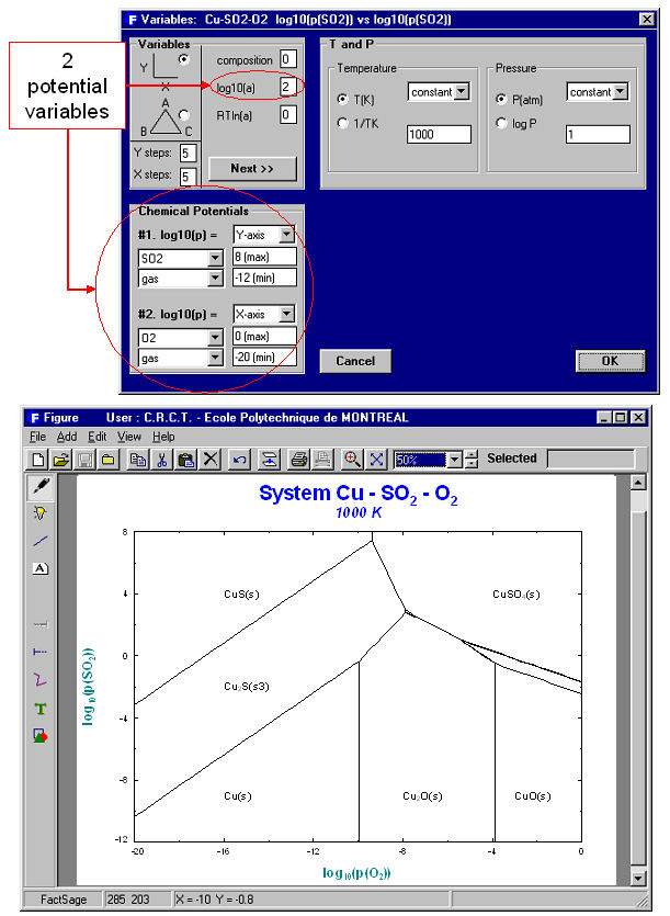
The
versatility of the choice of axes in the Variables
Window enables one to generate many different types
of phase diagrams. Fig. 4 is a classical isothermal predominance
area diagram for the Cu-SO2-O2 system.
The system components are Cu, SO2, O2;
the axis variables are log10(Pso2)
and log¨10(Po2) and the temperature
is set constant; the possible phases in the phase diagram
are gas and stoichiometric solids taken from the FACT
compound database. This diagram may be
compared to the one produced by the Predom
module for the same system.
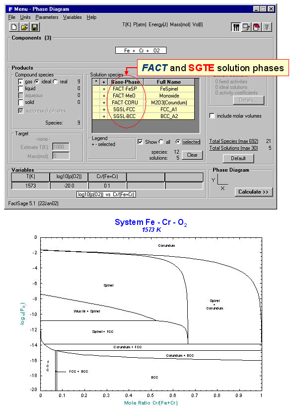
Unlike
the Predom
module, Phase Diagram
can produce predominance area diagrams that also include
data from the solution databases. Fig. 5 shows the log10(Po2)
vs Cr/(Cr+Fe) phase diagram at 1573 K where the system
components are Fe, Cr and O2. The possible
phases are the gas and various real solutions taken from
the FACT
(oxides) and SGTE
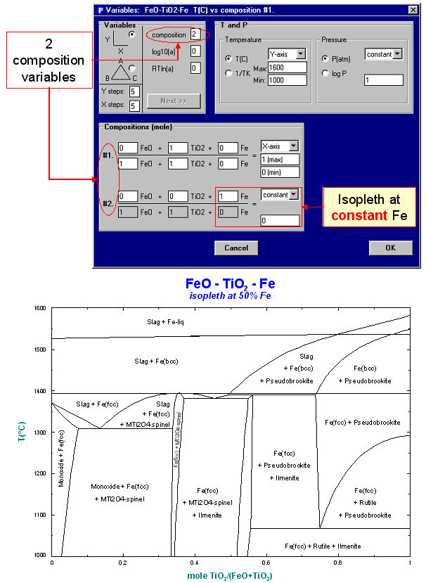
(alloys) databases. Fig. 6 is the input/output for an
isopleth of T(C) vs TiO2/(FeO+TiO2)
ratio at 50 mol % Fe in the FeO-TiO2-Fe system again using
both FACT
and SGTE
solution databases. An example of the interactive power
of Phase Diagram
is the equilibrium calculation shown in Fig. 7 where the
user has first selected the phase equilibrium mode
and then pointed and clicked at the coordinates 1450ºC
and TiO2/(FeO+TiO2) = 0.7. Note, these results
would be identical to a calculation with the Equilib
module at 1450ºC and 1 atm where the reactants are
0.7 TiO2 + 0.3 FeO + excess Fe.
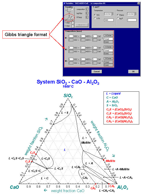
Fig. 8 is the input/output for a Gibbs ternary section
of the CaO–Al2O3–SiO2
system at 1600ºC using FACT
data.
The
calculated diagrams can be stored as figure (*.fig) files,
edited by the Figure
module, and exported as *.bmp, *.emf and *.wmf files.
Examples of the combined use of the Phase
Diagram, Equilib
and Figure
modules to generate phase diagrams are shown in figures
9 to 15.
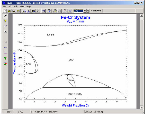
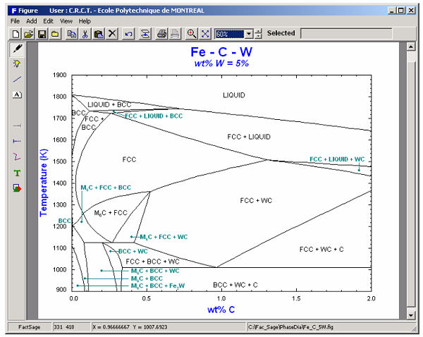
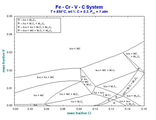
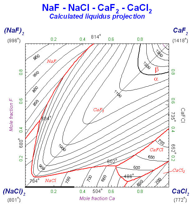
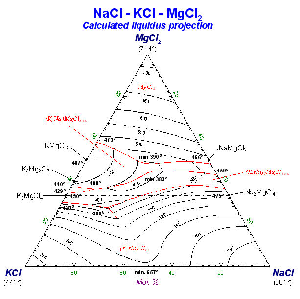
A
variety of calculated phase diagrams - some edited and
enhanced via the Figure
Module (labels added, etc.) – are shown in Figs
9 to 15.
;)
;)

;)
;)
;)
;)